Pseudotime Trajectory Inference#
![]()
^ Binder launches an interactive session of this tutorial with the environment pre-configured!
MIRA’s pseudotime facilities infer pseudotime and parse lineage trees from the joint k-nearest neighbors graph of multiome data. First, MIRA applies an adaptation of the Palantir algorithm to calculate diffusion pseudotime and terminal state probabilities for each cell. Then, MIRA applies a new lineage tree inference algorithm to reconstruct bicurcating tree structure of differentation data.
In this tutorial, we will use pseudotime trajectory inference to investigate the lineage structure of the hair follicle.
First, import packages and the data:
[1]:
import mira
import anndata
import scanpy as sc
import matplotlib.pyplot as plt
import seaborn as sns
import warnings
import matplotlib
matplotlib.rc('font',size=12)
warnings.simplefilter("ignore")

umap_kwargs = dict(
    add_outline=True, outline_width=(0.1,0), outline_color=('grey', 'white'),
    legend_fontweight=550, frameon = False, legend_fontsize=12
)

mira.datasets.PseudotimeTrajectoryInferenceTutorial()

data = anndata.read_h5ad('mira-datasets/shareseq.hair_follicle.joint_representation.h5ad')
mira.utils.pretty_sderr()
INFO:mira.datasets.datasets:Dataset already on disk.
INFO:mira.datasets.datasets:Dataset contents:
        * mira-datasets/shareseq.hair_follicle.joint_representation.h5ad
[1]:
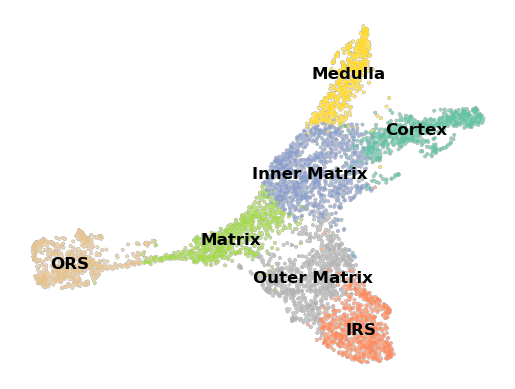
Taking a look at the UMAP, we see that starting from the ORS, cells progress through the Matrix, branching into the IRS, then the Cortex and Medulla.
[2]:
sc.pl.umap(data, color = 'true_cell', palette='Set2', legend_loc='on data', title = '', **umap_kwargs)
Defining pseudotime#
The first step in identifying the lineage structure of this data is to compute a diffusion map of the underlying nearest neighbors graph. sc.tl.diffmap will use the KNN graph in data.obsp["connectivities"] to compute a diffusion map representation of the data. In this case, the connectivities are derived from the Joint KNN graph, so the diffusion map will represent cells in a bimodal space.
First, calculate the diffusion map, then use mira.time.normalize_diffmap to rescale the components of the diffusion map. This regularizes distortions in magnitude of the eigenvectors.
[3]:
sc.tl.diffmap(data)
mira.time.normalize_diffmap(data)
INFO:root:Added key to obsm: X_diffmap, normalized diffmap with 14 components.
INFO:root:Added key to uns: eigen_gap
WARNING:root:Be sure to inspect the diffusion components to make sure they captured the heterogeniety of your dataset. Occasionally, the eigen_gap heuristic truncates the number of diffusion map components too early, leading to loss of variance.
Recommending 5 diffusion map components.
Next, we need to choose the best number of diffusion components to represent the data. Too few components will not capture the full structure of the data, too many will overfit and induce strange structures. Below, we use mira.pl.plot_eigengap to plot the “Eigengap” heuristic, which is the difference in magnitude of successive sorted eigenvalues.
The component with the highest Eigengap is an estimate of the best number of components to represent the data, but may not capture all relevent structure. For this reason, we also plot the diffusion components projected over the UMAP, with which we can check how many components are needed to capture differences between cell types.
In the case of the hair follicle, Eigengap recommends using 5 diffusion components, which appears to adequately describe differences bewteen cell types.
[4]:
mira.pl.plot_eigengap(data, palette='magma')
plt.show()


Next, we must define a new nearest-neighbors graph based on the diffusion components. For sc.pp.neighbors, we indicate that we wish to calculate a new KNN graph using the first 5 components from data.obsm["X_diffmap"].
It is critical that you subset how many components to use before calculating nearest neighbors on the diffusion map.
[6]:
data.obsm['X_diffmap'] = data.obsm['X_diffmap'][:,:5] # subset the number of dimensions
sc.pp.neighbors(data, use_rep='X_diffmap', key_added='X_diffmap')
Then, we check to make sure there are no disconnected component graphs in the data using mira.time.get_connected_components. The remainder of the methods only work on connected graphs, and will raise an error if they are run on cells spanning multiple disconnected components.
[7]:
mira.time.get_connected_components(data)
INFO:mira.pseudotime.pseudotime:Found 1 components of KNN graph.
INFO:mira.adata_interface.core:Added cols to obs: mira_connected_components
Now, we can assign cells a pseudotime and define a transport map describing a markov chain model of forward differentiation using mira.time.get_transport_map. This function requires we define a start cell, which must be chosen using knowledge of the system. Usually, the cell which is the minima or maxima of the first diffusion component works well as a start point. In this case, we use the minima:
[8]:
mira.time.get_transport_map(data, start_cell= int(data.obsm['X_diffmap'][:,0].argmax()))
INFO:mira.pseudotime.pseudotime:Calculating inter-cell distances ...
INFO:root:Using 1 core. Speed this up by allocating more n_jobs.
INFO:mira.pseudotime.pseudotime:Calculating transport map ...
INFO:mira.adata_interface.pseudotime:Added key to obs: mira_pseudotime
INFO:mira.adata_interface.pseudotime:Added key to obsp: transport_map
INFO:mira.adata_interface.pseudotime:Added key to uns: start_cell
This function calculates the transport map and assigns cells a pseudotime based on their shortest-path distance from the start cell:
[9]:
sc.pl.umap(data, color = 'mira_pseudotime', show = False,
           **umap_kwargs, color_map = 'magma')
... storing 'mira_connected_components' as categorical
[9]:
<AxesSubplot:title={'center':'mira_pseudotime'}, xlabel='UMAP1', ylabel='UMAP2'>

Lineage inference#
From the transport map, we may find terminal states where the markov chain reaches a steady state. mira.time.find_terminal_cells outputs cells that appear to be at the termini of lineages. Increase the iterations parameter, or increase the treshold parameter (e.g. 1e-3 to 1e-2) to find more terminal cell candidates. Be sure to set the seed for repeatable results.
[10]:
terminal_cells = mira.time.find_terminal_cells(data, seed = 3)
print('Terminal cells: ', ', '.join(terminal_cells))
MORE_terminal_cells = mira.time.find_terminal_cells(data, seed = 3, iterations = 10, threshold=1e-2)

fig, ax = plt.subplots(1,2,figsize=(15,5))
sc.pl.umap(data, color = 'mira_pseudotime', show = False,
           **umap_kwargs, color_map = 'magma', ax = ax[0])
sc.pl.umap(data[terminal_cells], na_color = 'black', ax = ax[0],
          size = 200, title = 'Terminal Cells', show=False)

sc.pl.umap(data, color = 'mira_pseudotime', show = False,
           **umap_kwargs, color_map = 'magma', ax = ax[1])
sc.pl.umap(data[MORE_terminal_cells], na_color = 'black', ax = ax[1],
           size = 200, title = 'MORE terminal Cells')
INFO:mira.pseudotime.pseudotime:Found 3 terminal states from stationary distribution.
Terminal cells: R1.18.R2.43.R3.02.P1.55, R1.23.R2.87.R3.61.P1.53, R1.64.R2.61.R3.40.P1.56
INFO:mira.pseudotime.pseudotime:Found 9 terminal states from stationary distribution.

Next, we use mira.time.get_branch_probabilities to find the probability of reaching each terminal state from each cell in the markov chain. To this function, we provide a dictionary with lineage names as keys, and values as terminal cell barcodes.
[11]:
mira.time.get_branch_probabilities(data, terminal_cells= {
    'Medulla' : terminal_cells[1],
    'Cortex' : terminal_cells[0],
    'IRS' : terminal_cells[2]
})
INFO:mira.pseudotime.pseudotime:Simulating random walks ...
INFO:mira.adata_interface.pseudotime:Added key to obsm: branch_probs
INFO:mira.adata_interface.pseudotime:Added key to uns: lineage_names
INFO:mira.adata_interface.core:Added cols to obs: Medulla_prob
INFO:mira.adata_interface.core:Added cols to obs: Cortex_prob
INFO:mira.adata_interface.core:Added cols to obs: IRS_prob
INFO:mira.adata_interface.core:Added cols to obs: differentiation_entropy
Outputs from this function include the probabilities of reaching each terminal state, and differentiation entropy.
[12]:
sc.pl.umap(data,
   color = [x + '_prob' for x in data.uns['lineage_names']],
   color_map='magma', **umap_kwargs)

Finally, we can parse the lineage probabilities to find the bifurcating tree structure of the data. The mira.time.get_tree_structure function takes the threshold parameter, which controls how sensitive the algorithm is to branch divergences.
Specifically, threshold controls the how great the log2-ratio of differentiating down one branch compared to another must be to declare a branch point. To place branch points when the probability of traveling down the Medulla branch is 1.5 times greater than the Cortex branch, set threshold to 0.58 (this appears to work as a good default):
[13]:
mira.time.get_tree_structure(data, threshold = 0.6)
sc.pl.umap(data, color = 'tree_states', palette = 'Set2',
           **umap_kwargs, title = '', legend_loc='on data')
INFO:mira.adata_interface.pseudotime:Added key to obs: tree_states
INFO:mira.adata_interface.pseudotime:Added key to uns: tree_state_names
INFO:mira.adata_interface.pseudotime:Added key to uns: connectivities_tree
... storing 'tree_states' as categorical

Visualizing lineages and topics#
Finally, with the tree structure solved, we can visualize expression dynamics using streamgraphs. For more information on making informative visualizations using this flexible interface, read the streamgraph docs and check out the streamgraph tutorial.
[14]:
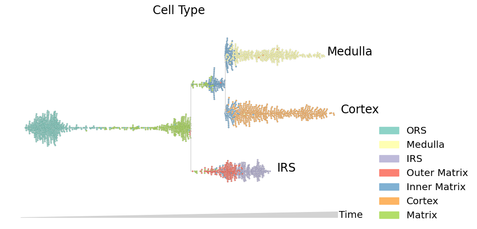
data.obs.true_cell = data.obs.true_cell.astype(str)
mira.pl.plot_stream(data, data = 'true_cell', log_pseudotime=False, max_bar_height=0.99, title = 'Cell Type',
figsize=(10,5), style = 'swarm', palette='Set3', size = 5, max_swarm_density = 100)
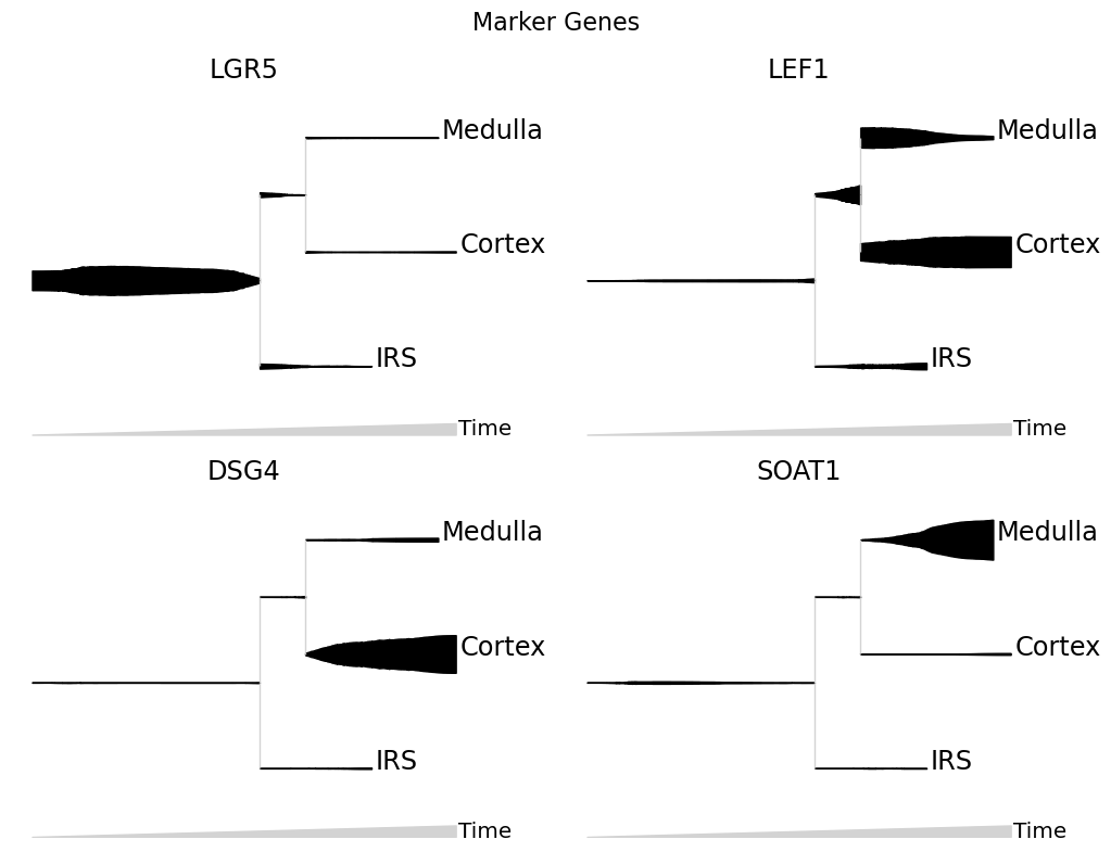
mira.pl.plot_stream(data, data = ['LGR5','LEF1','DSG4','SOAT1'],
log_pseudotime=False, layers = None, plots_per_row = 2,
clip = 3, window_size=301, scale_features=True, split = True,
title = 'Marker Genes')
plt.show()
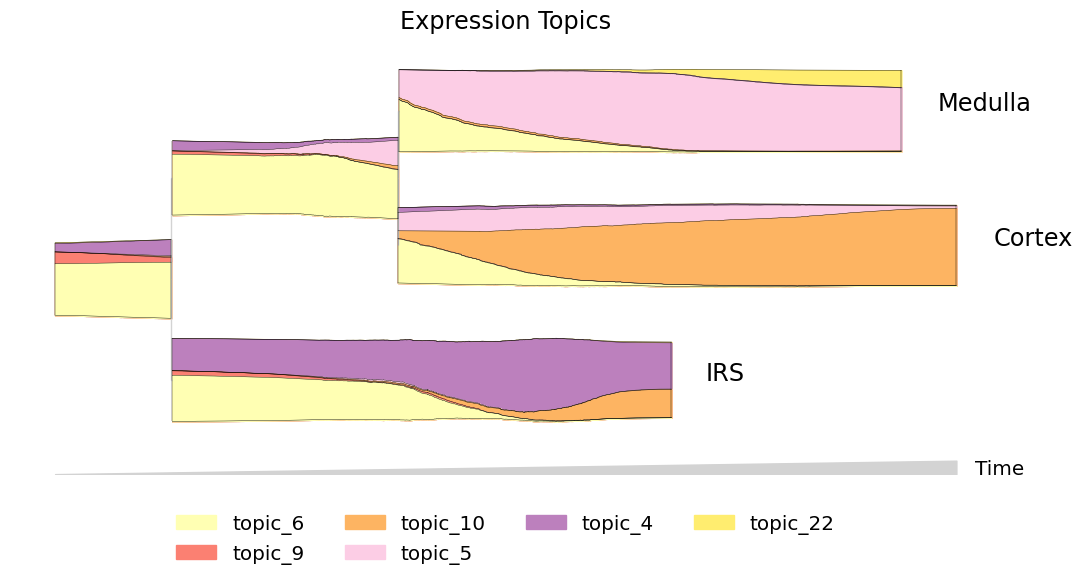
One of the most informative ways to explore pseudotemporal progressions is to visualize the flow of topics through lineages. Plot the flow of expression and accessibility topics side-by-side to compare which modes are driving major changes in cell-type identity:
[15]:
plot_kwargs = dict(hide_feature_threshold=0.03, linewidth=0.3, max_bar_height=0.8,
                    window_size=301, legend_cols=4, figsize = (11,6))

mira.pl.plot_stream(data[data.obs.mira_pseudotime > 6.5],
                    data = ['topic_' + str(i) for i in [6,9,10,5,4,22]],
                    title = 'Expression Topics',
                    palette=sns.color_palette('Set3')[1::2], # warm tones
                    **plot_kwargs)
[15]:
(<Figure size 1100x600 with 1 Axes>,
 <AxesSubplot:title={'center':'Expression Topics'}>)
[16]:
mira.pl.plot_stream(data[data.obs.mira_pseudotime > 6],
                    data = ['ATAC_topic_' + str(i) for i in [0, 15, 23, 17, 14, 21, 4]],
                    title = 'Accessibility Topics',
                    palette=sns.color_palette('Set3')[::2], #+ sns.color_palette('tab20')[::1], # cool tones
                    **plot_kwargs)
plt.show()
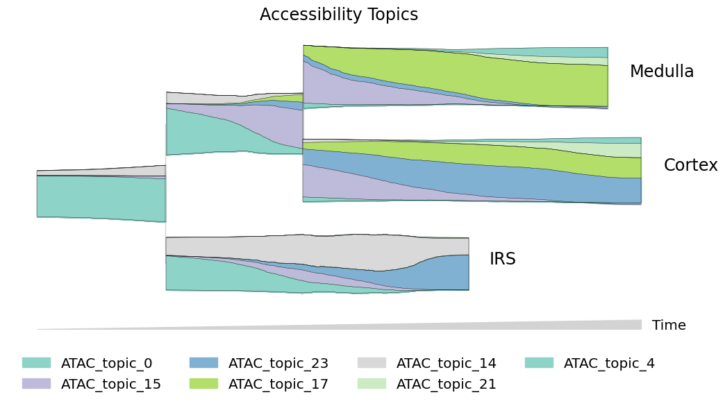
Side note: We like to use mostly warm tones to describe expression data and cool tones to describe accessibility data. One easy trick to do this with seaborn color palletes is to pass only even-numbered colors from the Set3 and Set2 palettes to accessibility streams, and only odd-numbered colors to expression streams.
Transport map tracing#
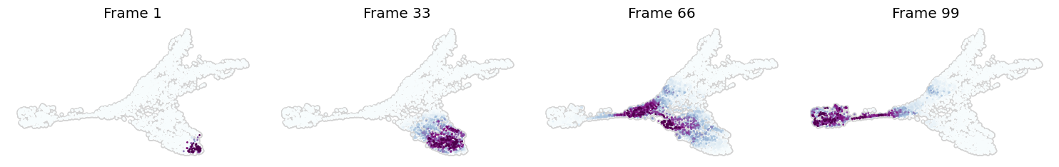
We can also simulate the differentiation process using mira.time.trace_differentiation. In this case, we may be interested in finding the ancestral populations of the IRS lineage.
This function traces the differentiation process through the diffusion map starting from user-defined start cells, and may be used to investigate complicated lineage structures that may violate the typical assumptions made during lineage inference (no cycles, one path to each termini, terminal states don’t regress, etc.)
We can start from a given start_lineage and work backwards, like below:
[17]:
!mkdir -p data
mira.time.trace_differentiation(data, start_lineage='IRS', num_steps=1500,
                               save_name='data/hf_diff.gif', direction='backward', sqrt_time=True,
                               log_prob=True, steps_per_frame=15, figsize=(7,5), ka=3)
INFO:mira.pseudotime.backtrace:Creating transport map ...
INFO:mira.pseudotime.backtrace:Tracing ancestral populations ...
INFO:mira.pseudotime.backtrace:Creating animation ...
INFO:mira.pseudotime.backtrace:Saving animation ...
INFO:matplotlib.animation:Animation.save using <class 'matplotlib.animation.PillowWriter'>
The function above makes a video of the process and prints out some preview frames. Then, it saves the video to save_name as a gif.
[18]:
mira.utils.show_gif('data/hf_diff.gif')

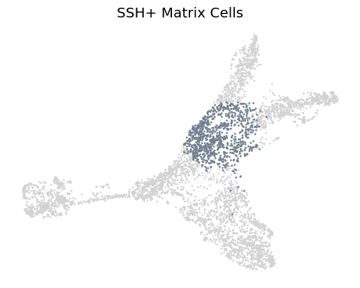
We may also run a forward simulation from an interesting group of cells to see their ancestral populations. In this case, we may want to see if the SSH+ matrix population can still generate the IRS population:
[19]:
ax = sc.pl.umap(data, show = False, size = 15)
sc.pl.umap(data[data.obs.true_cell == 'Inner Matrix'], na_color = 'slategrey', ax = ax,
          frameon=False, size = 15, title = 'SSH+ Matrix Cells')
... storing 'true_cell' as categorical
[20]:
mira.time.trace_differentiation(data,start_cells=data.obs.true_cell.values == 'Inner Matrix', num_steps=1301,
                               save_name='data/hf_diff.gif', direction='forward', sqrt_time=True,
                               log_prob=True, steps_per_frame=20, figsize=(7,5), ka = 3,
                               vmax_quantile=0.97)
INFO:mira.pseudotime.backtrace:Creating transport map ...
INFO:mira.pseudotime.backtrace:Tracing ancestral populations ...

INFO:mira.pseudotime.backtrace:Creating animation ...
INFO:mira.pseudotime.backtrace:Saving animation ...
INFO:matplotlib.animation:Animation.save using <class 'matplotlib.animation.PillowWriter'>
[21]:
mira.utils.show_gif('data/hf_diff.gif')

Yes! This consistent with experimental lineage tracing evidence that SSH+ matrix cells can differentiate into IRS cells. This also suggests that the pathway from SSH- and SSH+ matrix cells to the IRS cell type is distinct.
Overall, the parameters needed for pseudotime trajectory inference are:
Parameter |
Source |
What it does |
Good value |
|---|---|---|---|
threshold |
MIRA |
Controls how far the probability of progressing down one lineage at a branch must diverge from the probability of progressing down another branch before the branch point is assigned. Different topologies demand different thresholds. Try values to find appropriate branch points. |
0.2, 0.5, 1 |
num diffmap components |
MIRA |
Number of diffusion map components to use for transport map construction. Determined by eigengap heuristic |
determined by eigengap |
n_neighbors |
MIRA |
Number of neighbors each cell may transition to in the transport map. |
15, 30 |
ka |
MIRA |
Neighborhood size, for adaptive Gaussian kernel, the standard deviation is set as the distance to the kath neighbor |
5 |
Usually, threshold is the only parameter that must be adjusted.
Next, one of the most interesting aspects of analyzing multiomics data is constrasting the regulatory dynamics of cis-accessibility and gene expression over differentiation timecourses. Of particular interst is when these two related measures of cell state diverge. Please proceed to the next tutorial on Cis-regulatory modeling.