mira.pl.plot_stream#
- mira.pl.plot_stream(adata, data=None, layers=None, pseudotime_key='mira_pseudotime', group_key='tree_states', tree_graph_key='connectivities_tree', group_names_key='tree_state_names', style='stream', split=False, log_pseudotime=True, scale_features=False, order=None, title=None, show_legend=True, legend_cols=5, max_bar_height=0.6, size=None, max_swarm_density=100000.0, hide_feature_threshold=0, palette=None, color='black', linecolor='black', linewidth=None, hue_order=None, pseudotime_triangle=True, scaffold_linecolor='lightgrey', scaffold_linewidth=1, min_pseudotime=- 1, orientation='h', figsize=(10, 5), ax=None, plots_per_row=4, height=4, aspect=1.3, tree_structure=True, center_baseline=True, window_size=101, clip=10, alpha=1.0, vertical=False, enforce_max=None)#
Plot a streamgraph representation of a differentiation or continuous process. Modifying the parameters produces variations of the streamgraph for making different sorts of comparisons. The available modes are:
stream - 3 to 20 continous features
swarm - one discrete feature
line and scatter - comparing modalities for one feature
heatmap - 20 or more continous features, no lineage tree
Note
To plot a stream graph, you must first perform lineage inference on the data using the mira.time API.
- Parameters
- datalist[str] or str
Which data features of dataframe to plot. If str, plots one feature. If list, plots each feature. The feature may be the name of a gene or a cell-level attribute in the .obs dataFrame.
- layerslist[str] or str
Which layer of dataframe to plot for a given attribute. If str, all features provided in data will be found in the same layer. If list, must provide a list where each element is a layer that is the same length as data. For features that are in .obs, any layer name may be provided. To plot two attributes for the same gene, for example, expression and accessibility, list that gene twice in data, then specify the two layers to use.
- style{“stream”, “swarm”, “heatmap”, “line”, “scatter”}, default = “stream”
Style to plot data. The attributes and advantages of each style are outlined in the Notes section.
- scale_featuresboolean, default = False
Independently scale each feature to the range [0,1]. Enables comparisons of feature trends with different magnitudes.
- splitboolean, defaut = False
Whether to split each feature into its own plot. By default, stream, scatter, and line mode will plot multiple features on the same plot. Setting split to True will create a separate plot for each feature. This feature is not available for heatmaps, and is enforced behavior for swarms.
- order{“ascending”, “descending”, None}, default = None
Ascending order plots features in the order at which they peak in terms of pseudotime, so feature that peak earlier will appear first on the plot. Vice- versa for descending order. Setting order to None will plot features in the order they are provided to data.
- window_size{ i | i > 0, i is odd }, default = 101
Odd integer number. Used for smoothing of data for streams, lines, and scatter plots. Used as the number of cells to aggregate per column in heatmap mode. Increasing this parameter will produce smoother plots.
- clipfloat > 0, default = 10
Values of feature x are clipped to be within the bounds of mean(x) +/- clip * std(x). This trims in outliers and reduces their effect on smoothing. This is useful for noisy data.
- tree_structureboolean, default = True
Whether to plot the lineage tree structure of the data. This is disabled for heatmap mode. If set to False, this will not required that you have conducted lineage inference on the data, only that you have some sort of time assigned to each cell.
- Plot Aesthetics
- max_bar_heightfloat (0, 1), default = 0.6
The amount of space occupied by the stream/scatter/line/swarm at its maximum magnitude. A max_bar_height of 1 will fill all available space with no room between lineages.
- sizefloat > 0 or None, default = None
Size of dots for swarm or scatter plots. Default of None will use defaults from swarmplot and scatterplot sub functions.
- max_swarm_densityfloat > 0, default = 1e5
Maximum number of points per pseudotime on swarmplot. Reducing this parameter reduces the number of points to draw and speeds up plotting. This parameter may also be adjusted to prevent points from overflowing into the gutters of swarm segments.
- hide_feature_thresholdfloat >= 0, < 1, default = 0.
If a feature comprises less than this fraction of the magnitude of the plot at some timepoint, hide that feature. This is useful when plotting streams with many features, many of which are close to zero at any given time. Increasing this parameter above 0. will hide those features and declutter the plot.
- linewidthfloat > 0 or None, default = None
Width of elements colored by linecolor. Default of None differs to style-specific default values.
- scaffold_linewidthfloat > 0, default = 1
Linewidth of scaffold
- pseudotime_triangeboolean, default = True
Whether to plot the triange marking the pseudotime axis at bottom of plot.
- Pseudotime Options
- pseudotime_keystr, default = ‘mira_pseudotime’,
Which key in .obs to use for the pseudotime for each cell (x-axis of plot). Sometimes, the pseudotime calculated by the mira.time API may be inconvenient for plotting because segments of the lineage tree may have unweildy lengths. You can use your own pseudotime metric or transformation by specifying which column in .obs to find it.
- log_pseudotimeboolean, default = True
Diffusion pseudotime increases exponentially with distance from the root. Log pseudotime compresses the upper ranges of pseudotime and typically yields more balanced plots.
- min_pseudotimefloat > 0, default = 0.05
This parameter ensures no segment on the lineage tree is shorter in pseudotime than the value provided. If a certain segment of the lineage tree is too short to be visualized, it may be increased.
- Coloring
- palettestr, list[str], or None; default = None
Palette of plot. Default of None will set palette to the style-specific default.
- colorstr, default = “black”
When only plotting one feature, streams, lines, or scatters, are colored by this parameter rather than palette. This behavior is similar to matplotlib.
- linecolorstr, default = “black”
Color of edges of plots, including outline of streams, scatters, and swarms.
- scaffold_linecolorstr, default = “lightgrey”
Color of lineage tree scaffold
- hue_orderlist[str] or None, default = None
Order to assign hues to features provided by data. Works similarly to hue_order in seaborn. User must provide list of features corresponding to the order of hue assignment.
- Plot Specifications
- titlestr or None, default = None
Title of figure
- show_legendboolean, default = True
Show figure legend
- legend_colsint, default = 5
Number of columns for horizontal legend.
- figsizetuple(float, float), default = (7,4)
Size of figure
- axmatplotlib.pyplot.axes, deafult = None
Provide axes object to function to add streamplot to a subplot composition, et cetera. If no axes are provided, they are created internally.
- plots_per_rowint > 0, default = 4
Number of plots per row when in swarm mode or when split is True.
- heightflaot > 0, default = 4
Height of plot when split. Otherwise, function uses figsize.
- aspectfloat > 0, default 1.3
Apsect ratio of split plots
- Other Parameters
- alphafloat in [0,1], defaut = 1
Transparency of plot elements.
- verticalboolean, default = False
Does not currently do anything.
- tree_graph_keystr, deafult = ‘connectivities_tree’,
Which key in .uns to find the connectivities tree between lineage tree segments. Contains a np.ndarray of shape (2*n_tree_states - 1, 2*n_tree_states - 1) with elements equal to one at index i,j meaning tree_state j is a descendent of i. This is found by mira.time.get_tree_structure, but may be manually encoded.
- group_names_key = ‘tree_state_names’,
Which key in .uns to find the names of the tree states corresponding to columns and rows of tree_graph_key.
- group_key = ‘tree_states’,
Which column in .obs to find the cell membership to particular tree states.
Examples
Note
Below, we provide a smattering of examples. For a more in-depth tutorial, see the streamgraph tutorial.
Plotting topics. Plot the composition of topics along a differentiation. Here hide_feature_threshold hides topics which aren’t contributing to the cell composition. This significantly cleans up the plot.
>>> topics = [6,9,10,5,4,22]
>>> mira.pl.plot_stream(data, data = ["topic_" + str(i) for i in topics], style = "stream",
...     hide_feature_threshold = 0.03, window_size = 301, max_bar_height = 0.8, order = 'ascending',
...     palette = "Set3", legend_cols = 3, log_pseudotime = False, linewidth=0.3)
>>> plt.show()

Comparing expression and accessibility. We provide the gene “LEF1” to data twice, then indicate to MIRA to plot the expression, then accessibility of “LEF1”. We set order to None so that the provided palette always matches with the correct mode. We also set scale_features to True so that we can compare trends instead of absolute magnitudes.
>>> mira.pl.plot_stream(data, data = ["LEF1","LEF1"], style = "line",
...    layers = ["expression","accessibility"], window_size = 301, max_bar_height = 0.8,
...    palette = ["red","black"], order = None, scale_features = True, figsize=(5,3),
...    clip = 3, log_pseudotime = False)
>>> plt.show()

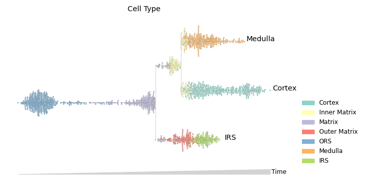
Plotting cluster membership using swarm mode. Swarm mode is useful for plotting discrete features.
>>> mira.pl.plot_stream(data, data = "true_cell", style = "swarm", palette = "Set3",
...     max_swarm_density = 100, max_bar_height = 0.8, size = 5, log_pseudotime = False)
>>> plt.show()
Visualizing marker genes. Each gene is plotted on its own stream.
>>> mira.pl.plot_stream(data, data = ["LEF1","WNT3","CTSC","LGR5"], style = "stream",
...     color = "black", split = True, clip = 2, scale_features=True,
...     log_pseudotime = False, window_size = 301)
>>> plt.show()

Using heatmap mode. Note that heatmap mode does not contain lineage tree information, so it is best to subset the tree down to one lineage. You can do this by subsetting the input data to only contain cells along the path you want to see.
Below, the boolean mask adata.obs.tree_states.str.contains(“Cortex”) selects for cells whose tree_state attribute indicates that cell is upstream of the cortex lineage.
>>> mira.pl.plot_stream(data[data.obs.tree_states.str.contains("Cortex")],
...     data = ["LGR5","EDAR","LEF1","WNT3"], style = "heatmap", order = None,
...     window_size = 101, scale_features=True, tree_structure = False, figsize=(7,3),
...     log_pseudotime = False)
>>> plt.show()

You can subset cells using more complicated filters. For example, to include only cells which may differentiate into Cortex or Medulla cells:
>>> mira.pl.plot_stream(data[data.obs.tree_states.str.contains("Cortex|Medulla")],
...     data = ["DSG4","SOAT1","LEF1"], style = "stream", window_size = 301,
...     scale_features = True, palette='Set2', linewidth=0.5, clip = 1,
...     max_bar_height = 0.99)
>>> plt.show()

Finally, you can create plots without lineage structure by setting tree_structure to False. This creates a more traditional 2-dimensional plot, showing, for example, the levels of Lgr5 and Lef1 along the path from ORS to Cortex cells:
>>> mira.pl.plot_stream(data[data.obs.tree_states.str.contains('Cortex')],
...     data = ['LEF1','LGR5'], log_pseudotime=False, title = 'Gene Counts',
...     style = 'scatter', window_size = 301, tree_structure=False,
...     palette=['black','red'], max_bar_height=0.99, size = 3)
>>> plt.show()
