mira.topics.AccessibilityTopicModel

class mira.topics.AccessibilityTopicModel(*args, **kwargs)

Generic class for topics models for analyzing chromatin accessibility data. All accessibility topic models inherit from this class and implement the same methods.

Methods

fit(adata_or_dirname[, writer, reinit, ...])	Initializes new weights, then fits model to data.
get_enriched_TFs(adata[, factor_type, ...])	Get TF enrichments in top peaks associated with a topic.
get_enrichments(topic_num[, factor_type])	Returns TF enrichments for a certain topic.
get_hierarchical_umap_features(adata[, key, ...])	Leverage the hiearchical relationship between topic-feature distributions to prduce a balance matrix for isometric logratio transformation.
get_learning_rate_bounds(adata_or_dirname[, ...])	Use the learning rate range test (LRRT) to determine minimum and maximum learning rates that enable the model to traverse the gradient of the loss.
get_motif_scores(adata[, factor_type, ...])	Get motif scores for each cell based on the probability of sampling a motif from the posterior distribution over accessible sites in a cell.
get_umap_features(adata[, key, box_cox, add_key])	Predict transformed topic compositions for each cell to derive nearest- neighbors graph.
impute(adata[, key, batch_size, bar, ...])	Impute the relative frequencies of features given the cells' topic compositions.
instantiate_model(adata_or_dirname)	Given the exogenous and enxogenous features provided, instantiate weights of neural network.
load(filename)	Load a pre-trained topic model from disk.
plot_compare_topic_enrichments(topic_1, topic_2)	It is often useful to contrast topic enrichments in order to understand which factors' influence is unique to certain cell states.
plot_learning_rate_bounds([figsize, ax, ...])	Plot the loss vs.
predict(adata_or_dirname[, batch_size, bar, ...])	Predict the topic compositions of cells in the data.
save(filename)	Save topic model.
score(adata_or_dirname[, batch_size])	Get normalized ELBO loss for data.
set_device(device)	Move topic model to a new device.
set_learning_rates(min_lr, max_lr)	Set the lower and upper learning rate bounds for the One-cycle learning rate policy.
to_cpu()	Move topic model to CPU device "cpu", if available.
to_gpu()	Move topic model to GPU device "cuda:0", if available.
trim_learning_rate_bounds([...])	Adjust the learning rate boundaries for the One-cycle learning rate policy.

rank_peaks

get_learning_rate_bounds(adata_or_dirname, num_steps=100, eval_every=3, num_epochs=3, lower_bound_lr=1e-06, upper_bound_lr=5)

Use the learning rate range test (LRRT) to determine minimum and maximum learning rates that enable the model to traverse the gradient of the loss.

Steps through linear increase in log-learning rate from lower_bound_lr to upper_bound_lr while recording loss of model. Learning rates which produce greater decreases in model loss mark range of possible learning rates.

Parameters

adataanndata.AnnData

AnnData of expression or accessibility features to model

num_stepsint, default=100

Number of steps to run the LRRT.

eval_everyint, default=3,

Aggregate this number of batches per evaluation of the objective loss. Larger numbers give lower variance estimates of model performance.

lower_bound_lrfloat, default=1e-6

Start learning rate of LRRT

upper_bound_lrfloat, default=5

End learning rate of LRRT

Returns

min_learning_ratefloat

Lower bound of estimated range of optimal learning rates

max_learning_ratefloat

Upper bound of estimated range of optimal learning rates

Examples

>>> model.get_learning_rate_bounds(rna_data, num_epochs = 3)
Learning rate range test: 100%|██████████| 85/85 [00:17<00:00,  4.73it/s]
(4.619921114045972e-06, 0.1800121741235493)

set_learning_rates(min_lr, max_lr)

Set the lower and upper learning rate bounds for the One-cycle learning rate policy.

Parameters

min_lrfloat

Lower learning rate boundary

max_lrfloat

Upper learning rate boundary

Returns

None

trim_learning_rate_bounds(lower_bound_trim=0.0, upper_bound_trim=0.5)

Adjust the learning rate boundaries for the One-cycle learning rate policy. The lower and upper bounds should span the learning rates with the greatest downwards slope in loss.

Parameters

lower_bound_trimfloat>=0, default=0.

Log increase in learning rate of lower bound relative to estimated boundary given from LRRT. For example, if the estimated boundary by LRRT is 1e-4 and user gives `lower_bound_trim`=1, the new lower learning rate bound is set at 1e-3.

upper_bound_trimfloat>=0, default=0.5,

Log decrease in learning rate of upper bound relative to estimated boundary give from LRRT.

Returns

min_learning_ratefloat

Lower bound of estimated range of optimal learning rates

max_learning_ratefloat

Upper bound of estimated range of optimal learning rates

Examples

>>> model.trim_learning_rate_bounds(2, 1)
(4.619921114045972e-04, 0.1800121741235493e-1)

plot_learning_rate_bounds(figsize=(10, 7), ax=None, show_spline=True)

Plot the loss vs. learning rate curve generated by the LRRT test with the current boundaries.

Parameters

figsizetuple(int, int), default=(10,7)

Size of the figure

axmatplotlib.pyplot.axes or None, default = None

Pre-supplied axes for plot. If None, will generate new axes

Returns

axmatplotlib.pyplot.axes

Examples

When setting the learning rate bounds for the topic model, first run the LLRT test with get_learning_rate_bounds. Then, set the bounds on their respective ends of the part of the LRRT plot with the greatest slope, like below.

>>> model.trim_learning_rate_bounds(5,1) # adjust the bounds
>>> model.plot_learning_rate_bounds()

If the LRRT line appears to vary cyclically, that means your batches may be not be independent of each other (perhaps batches later in the epoch are more similar to eachother and more difficult than earlier batches. If this happens, randomize the order of your input data using.

instantiate_model(adata_or_dirname)

Given the exogenous and enxogenous features provided, instantiate weights of neural network. Called internally by fit.

Parameters

adataanndata.AnnData

AnnData of expression or accessibility features to model

Returns

selfobject

fit(adata_or_dirname, writer=None, reinit=True, log_every=10)

Initializes new weights, then fits model to data.

Parameters

adataanndata.AnnData

AnnData of expression or accessibility features to model

writertorch.utils.tensorboard.SummarWriter object or mira.topics.Writer object

Tracks per-batch loss metrics during training. The tensorboard object writes tensorboard log files, which can be visualized using TensorBoard. The MIRA Writer just tracks values in an in-memory dictionary.

log_everyint, default = 10

Average the batch metrics every “log_every” steps.

reinitbooleandefault = True

If fitting an already-trained model, whether to re-initialize weights with random values or keep the existing weights.

Returns

selfobject

Fitted topic model

Note

Fitting a topic model usually takes a 2-5 minutes for the expression model and 5-10 minutes for the accessibility model for a typical experiment (5K to 40K cells).

Tuning the topic model hyperparameters, however, can take longer. Finding the best number of topics significantly increases the interpretability of the model and its faithfullness to the underlying biology and is well worth the wait. To learn about topic model tuning, see mira.topics.TopicModelTuner.

predict(adata_or_dirname, batch_size=256, bar=True, box_cox=0.25, add_key='X_topic_compositions', add_cols=True, col_prefix='topic_')

Predict the topic compositions of cells in the data. Adds the topic compositions to the .obsm field of the adata object.

Parameters

adataanndata.AnnData

AnnData of expression or accessibility features to model

batch_sizeint>0, default=512

Minibatch size to run cells through encoder network to predict topic compositions. Set to highest value where tensors will fit in memory to increase speed.

Returns

adataanndata.AnnData

.obsm[‘X_topic_compositions’]np.ndarray[float] of shape (n_cells, n_topics)

Topic compositions of cells

.obsm[‘X_umap_features’]np.ndarray[float] of shape (n_cells, n_topics)

ILR transformed topic embeddings for use with nearest neighbors graph

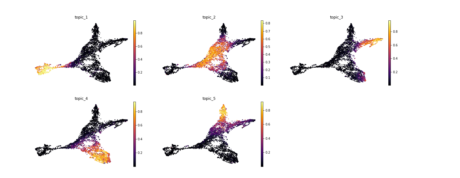
.obs[‘topic_1’] … .obs[‘topic_N’]np.ndarray[float] of shape (n_cells,)

Columns for the activation of each topic.

Examples

>>> model.predict(adata)
Predicting latent vars: 100%|█████████████████████████| 36/36 [00:03<00:00,  9.29it/s]
INFO:mira.adata_interface.topic_model:Added key to obsm: X_topic_compositions
INFO:mira.adata_interface.topic_model:Added cols: topic_1, topic_2, topic_3, 
topic_4, topic_5
>>> scanpy.pp.neighbors(adata, metric = "manhattan", use_rep = "X_umap_features")
>>> scanpy.tl.umap(adata, min_dist 0.1)
>>> scanpy.pl.umap(adata, color = model.topic_cols, **mira.pref.topic_umap(ncols = 3))

get_hierarchical_umap_features(adata, key='X_topic_compositions', dendogram_key='topic_dendogram', box_cox=0.5, *, add_key='X_umap_features')

Leverage the hiearchical relationship between topic-feature distributions to prduce a balance matrix for isometric logratio transformation. The function get_umap_features uses an arbitrary balance matrix that does not account for the relationship between topics.

The “UMAP features” are the transformation of the topic compositions that encode biological similarity in the high-dimensional space. Use those features to produce a joint KNN graph for downstream analysis using UMAP, clustering, and pseudotime inference.

Parameters

adataanndata.AnnData

AnnData of expression or accessibility features to model

box_cox“log” or float between 0 and 1

Constant for box-cox transformation of topic compositions

Returns

adataanndata.AnnData

.obsm[‘X_umap_features’]np.ndarray[float] of shape (n_cells, n_topics)

Transformed topic compositions of cells

.uns[‘topic_dendogram’]np.ndarray

linkage matrix given by scipy.cluster.hierarchy.linkage of hiearchical relationship between topic-feature distributions. Hierarchy calculated by hellinger distance and ward linkage.

Examples

>>> model.get_hierarchical_umap_features(adata) # to make features
INFO:mira.adata_interface.topic_model:Fetching key X_topic_compositions from obsm
INFO:mira.adata_interface.core:Added key to obsm: X_umap_features
INFO:mira.adata_interface.topic_model:Added key to uns: topic_dendogram
>>> scanpy.pp.neighbors(adata, metric = "manhattan", use_rep = "X_umap_features") # to make KNN graph

get_umap_features(adata, key='X_topic_compositions', box_cox=0.5, *, add_key='X_umap_features')

Predict transformed topic compositions for each cell to derive nearest- neighbors graph. Projects topic compositions to orthonormal space using isometric logratio transformation.

The “UMAP features” are the transformation of the topic compositions that encode biological similarity in the high-dimensional space. Use those features to produce a joint KNN graph for downstream analysis using UMAP, clustering, and pseudotime inference.

Parameters

adataanndata.AnnData

AnnData of expression or accessibility features to model

box_cox“log” or float between 0 and 1

Constant for box-cox transformation of topic compositions

Returns

adataanndata.AnnData

.obsm[‘X_umap_features’]np.ndarray[float] of shape (n_cells, n_topics)

Transformed topic compositions of cells

Examples

>>> model.get_umap_features(adata) # to make features
INFO:mira.adata_interface.topic_model:Fetching key X_topic_compositions from obsm
INFO:mira.adata_interface.core:Added key to obsm: X_umap_features
>>> scanpy.pp.neighbors(adata, metric = "manhattan", use_rep = "X_umap_features") # to make KNN graph

score(adata_or_dirname, batch_size=256)

Get normalized ELBO loss for data. This method is only available on topic models that have not been loaded from disk.

Parameters

adataanndata.AnnData

AnnData of expression or accessibility features to model

batch_sizeint>0, default=512

Minibatch size to run cells through encoder network to predict topic compositions. Set to highest value where tensors will fit in memory to increase speed.

Returns

lossfloat

Raises

AttributeError

If attempting to run after loading from disk or before training.

Notes

The score method is only available after training a topic model. After saving and writing to disk, this function will no longer work.

Examples

>>> model.score(rna_data)
0.11564

impute(adata, key='X_topic_compositions', batch_size=256, bar=True, add_layer='imputed', sparse=False)

Impute the relative frequencies of features given the cells’ topic compositions. The value given is rho (see manscript for details).

Parameters

adataanndata.AnnData

AnnData of expression or accessibility features to model

batch_sizeint>0, default=512

Minibatch size to run cells through encoder network to predict topic compositions. Set to highest value where tensors will fit in memory to increase speed.

Returns

anndata.AnnData

.layers[‘imputed’]np.ndarray[float] of shape (n_cells, n_features)

Imputed relative frequencies of features

Examples

>>> model.impute(rna_data)
>>> rna_data
View of AnnData object with n_obs × n_vars = 18482 × 22293
    layers: 'imputed'

save(filename)

Save topic model.

Parameters

filenamestr

File name to save topic model, recommend .pth extension

to_gpu()

Move topic model to GPU device “cuda:0”, if available.

to_cpu()

Move topic model to CPU device “cpu”, if available.

set_device(device)

Move topic model to a new device.

Parameters

devicestr

Name of device on which to allocate model

classmethod load(filename)

Load a pre-trained topic model from disk.

Parameters

filenamestr

File name of saved topic model

Examples

>>> rna_model = mira.topics.ExpressionTopicModel.load('rna_model.pth')
>>> atac_model = mira.topics.AccessibilityTopicModel.load('atac_model.pth')

get_enriched_TFs(adata, factor_type='motifs', mask_factors=True, binarize=True, top_quantile=0.2, *, topic_num)

Get TF enrichments in top peaks associated with a topic. Can be used to associate a topic with either motif or ChIP hits from Cistrome’s collection of public ChIP-seq data.

Before running this function, one must run either: mira.tl.get_motif_hits_in_peaks

or: mira.tl.get_ChIP_hits_in_peaks

Parameters

factor_typestr, ‘motifs’ or ‘chip’, default = ‘motifs’

Which factor type to use for enrichment

top_quantilefloat > 0, default = 0.2

Top quantile of peaks to use to represent topic in fisher exact test.

topic_numint > 0

Topic for which to get enrichments

Examples

>>> mira.tl.get_motif_hits_in_peaks(atac_data, genome_fasta = '~/genome.fa')
>>> atac_model.get_enriched_TFs(atac_data, topic_num = 10)

get_motif_scores(adata, factor_type='motifs', mask_factors=True, key='X_topic_compositions', batch_size=512, *, extra_features, covariates)

Get motif scores for each cell based on the probability of sampling a motif from the posterior distribution over accessible sites in a cell.

Parameters

adataanndata.AnnData

AnnData of accessibility features, annotated with TF binding using mira.tl.get_motif_hits_in_peaks or mira.tl.get_ChIP_hits_in_peaks.

batch_sizeint>0, default=512

Minibatch size to calculate posterior distribution over accessible regions. Only affects the amount of memory used.

factor_typestr, ‘motifs’ or ‘chip’, default = ‘motifs’

Which factor type to use for enrichment.

Returns

motif_scoresanndata.AnnData of shape (n_cells, n_factors)

AnnData object. For each cell from the original adata, gives score for each motif/ChIP factor.

get_enrichments(topic_num, factor_type='motifs')

Returns TF enrichments for a certain topic.

Parameters

topic_numint

For which topic to return results

factor_typestr, ‘motifs’ or ‘chip’, default = ‘motifs’

Which factor type to use for enrichment

Returns

topic_enrichmentslist[dict]

For each record, gives a dict of {‘factor_id’ : <id>, ‘name’ : <name>, ‘parsed_name’ : <name used for expression lookup>, ‘pval’ : <pval>, ‘test_statistic’ : <statistic>}

Raises

KeyErrorif get_enriched_TFs was not yet run for the given topic.

plot_compare_topic_enrichments(topic_1, topic_2, factor_type='motifs', label_factors=None, hue=None, palette='coolwarm', hue_order=None, ax=None, figsize=(8, 8), legend_label='', show_legend=True, fontsize=13, pval_threshold=(1e-50, 1e-50), na_color='lightgrey', color='grey', label_closeness=3, max_label_repeats=3, show_factor_ids=False)

It is often useful to contrast topic enrichments in order to understand which factors’ influence is unique to certain cell states. Topics may be enriched for constitutively-active transcription factors, so comparing two similar topics to find the factors that are unique to each elucidates the dynamic aspects of regulation between states.

This function contrasts the enrichments of two topics.

Parameters

topic1, topic2int

Which topics to compare.

factor_typestr, ‘motifs’ or ‘chip’, default = ‘motifs’

Which factor type to use for enrichment.

label_factorslist[str], np.ndarray[str], None; default=None

List of factors to label. If not provided, will label all factors that meet the p-value thresholds.

huedict[str{str, float}] or None

If provided, colors the factors on the plot. The keys of the dict must be the names of transcription factors, and the values are the associated data to map to colors. The values may be categorical, e.g. cluster labels, or scalar, e.g. expression values. TFs not provided in the dict are colored as na_color.

palettestr, list[str], or None; default = None

Palette of plot. Default of None will set palette to the style-specific default.

hue_orderlist[str] or None, default = None

Order to assign hues to features provided by data. Works similarly to hue_order in seaborn. User must provide list of features corresponding to the order of hue assignment.

axmatplotlib.pyplot.axes, deafult = None

Provide axes object to function to add streamplot to a subplot composition, et cetera. If no axes are provided, they are created internally.

figsizetuple(float, float), default = (8,8)

Size of figure

legend_labelstr, None

Label for legend.

show_legendboolean, default=True

Show figure legend.

fontsizeint>0, default=13

Fontsize of TF labels on plot.

pval_thresholdtuple[float, float], default=(1e-50, 1e-50)

Threshold below with TFs will not be labeled on plot. The first and second positions relate p-value with respect to topic 1 and topic 2.

na_colorstr, default=’lightgrey’

Color for TFs with no provided hue

colorstr, default=’grey’

If hue not provided, colors all points on plot this color.

label_closenessint>0, default=3

Closeness of TF labels to points on plot. When label_closeness is high, labels are forced to be very close to points.

max_label_repeatsboolean, default=3

Some TFs have multiple ChIP samples or Motif PWMs. For these factors, label the top max_label_repeats examples. This prevents clutter when many samples for the same TF are close together. The rank of the sample for each TF is shown in the label as “<TF name> (<rank>)”.

Returns

matplotlib.pyplot.axes

Examples

>>> label = ['LEF1','HOXC13','MEOX2','DLX3','BACH2','RUNX1', 'SMAD2::SMAD3']
>>> atac_model.plot_compare_topic_enrichments(23, 17,
...     label_factors = label, 
...     color = 'lightgrey',
...     fontsize=20, label_closeness=5, 
... )

previous

mira.topics.ExpressionTopicModel

next

mira.topics.BayesianTuner